|
M. Montes y Gómez, A. Gelbukh, A. López López, Ricardo Baeza-Yates. Flexible Comparison of Conceptual Graphs. In: Mayr, H.C., Lazansky, J., Quirchmayr, G., Vogel, P. (Eds.),Proc. DEXA-2001, 12th International Conference and Workshop on Database and Expert Systems Applications. Lecture Notes in Computer Science, N 2113,Springer-Verlag, 2001, pp. 102-111. |
|
|
|
|
Flexible Comparison of Conceptual Graphs*
1Center for Computing Research (CIC), National Polytechnic Institute (IPN), 07738, Mexico.
mmontesg@susu.inaoep.mx, gelbukh(?)cic.ipn.mx
2 Instituto Nacional de Astrofísica, Optica y Electrónica (INAOE), Mexico.
allopez@inaoep.mx
3 Departamento de Ciencias de la Computación, Universidad de Chile, Chile.
rbaeza@dcc.uchile.cl
Abstract. Conceptual graphs allow for powerful and computationally affordable representation of the semantic contents of natural language texts. We propose a method of comparison (approximate matching) of conceptual graphs. The method takes into account synonymy and subtype/supertype relationships between the concepts and relations used in the conceptual graphs, thus allowing for greater flexibility of approximate matching. The method also allows the user to choose the desirable aspect of similarity in the cases when the two graphs can be generalized in different ways. The algorithm and examples of its application are presented. The results are potentially useful in a range of tasks requiring approximate semantic or another structural matching – among them, information retrieval and text mining.
1. Introduction
In many application areas of text processing – e.g., in information retrieval and text mining – simple and shallow representations of the texts are commonly used. On one hand, such representations are easily extracted from the texts and easily analyzed, but on the other hand, they restrict the precision and the diversity of the results.
Recently, in all text-oriented applications there is a tendency to use richer representations than just keywords, i.e., representations with more types of textual elements. Under this circumstance, it is necessary to have the appropriate methods for the comparison of two texts in any of these new representations.
In this paper, we consider the representation of the texts by conceptual graphs [9,10] and focus on the design of a method for comparison of two conceptual graphs. This is a continuation of the research reported in [15].
Most methods for comparison of conceptual graphs come from information retrieval research. Some of them are restricted to the problem of determining if a graph, say, the query graph, is completely contained in the other one, say, the document graph [2,4]; in this case neither description nor measure of their similarity is obtained. Some other, more general methods, do measure the similarity between two conceptual graphs, but they typically describe this similarity as the set of all their common elements allowing duplicated information [3,6,7]. Yet other methods are focused on question answering [12]; these methods allow a flexible matching of the graphs, but they do not compute any similarity measure.
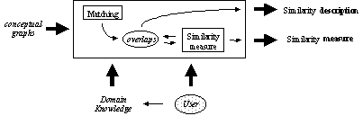
The method we propose is general but flexible. First, it allows measuring the similarity between two conceptual graphs as well as constructing a precise description of this similarity. In other words, this method describes the similarity between two conceptual graphs both quantitatively and qualitatively. Second, it uses domain knowledge – a thesaurus and a set of is-a hierarchies – all along the comparison process, which allows considering non-exact similarities. Third, it allows visualizing the similarities between two conceptual graphs from different points of view and selecting the most interesting one according to the user’s interests.
The paper is organized as follows. The main notions concerning conceptual graphs are introduced in section 2. Our method for comparison of two conceptual graphs is described in section 3, matching of conceptual graphs being discussed in subsection 3.1 and the similarity measure in subsection 3.2. An illustrative example is shown in section 4, and finally, some conclusions are discussed in the section 5.
2. Conceptual Graphs
This section introduces well-known notions and facts about conceptual graphs.
A conceptual graph is a finite oriented connected bipartite graph [9,10]. The two different kinds of nodes of this bipartite graph are concepts and relations.
Concepts represent entities, actions, and attributes. Concept nodes have two attributes: type and referent. Type indicates the class of the element represented by the concept. Referent indicates the specific instance of the class referred to by the node. Referents may be generic or individual.
Relations show the inter-relationships among the concept nodes. Relation nodes also have two attributes: valence and type. Valence indicates the number of the neighbor concepts of the relation, while the type expresses the semantic role of each one.
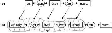
Figure 1 shows a simple conceptual graph. This graph represents the phrase “Tom is chasing a brown mouse”. It has three concepts and three relations. The concept [cat: Tom] is an individual concept of the type cat (a specific cat Tom), while the concepts [chase] and [mouse] are generic concepts. All relations in this graph are binary. For instance, the relation (attr) for attribute indicates that the mouse has brown color. The other two relations stand for agent and patient of the action [chase].
|
Figure 1. A simple conceptual graph |
Building and manipulating conceptual graphs is mainly based on six canonical rules [9]. Two of these rules are the generalization rules: unrestrict and detach.
Unrestrict rule generalizes a conceptual graph by unrestricting one of it concepts either by type or referent. Unrestriction by type replaces the type label of the concept with some its supertype; unrestriction by referent substitutes individual referents by generic ones.
Detach rule splits a concept node into two different nodes having the same attributes (type and referent) and distributes the relations of the original node between the two resulting nodes. Often this operation leads to separating the graph into two unconnected parts.
A conceptual graph v derivable from the graph u byapplying a sequence of generalization rules is called a generalization of the graph u; this is denoted as u £ v. In this case there exists a mapping p: v ® u with the following properties (pv is a subgraph of u called a projection of v in u; see Figure 2):[1]
· For each concept c in v, pc is a concept in pv such that type(pc) £ type(c). If c is an individual concept, then referent(pc) = referent(c).
· For each relation node r in v, pr is a relation node in pv such that type(pr) = type(r). If the i-th arc of r is linked to a concept c in v then the i-th arc of pr must be linked to pc in pv.
|
Figure 2. Projection mapping p: v ® u |
The mapping p is not necessarily one-to-one, i.e., two different concepts or relations can have the same projections (x1 ¹ x2 and px1 = px2, such situation results from application of detach rule). In addition, it is not necessarily unique, i.e., a conceptual graph v can have two different projections p and p´ in u, p´v¹pv.
If u1, u2, and v are conceptual graphs such that u1 £ v and u2 £ v, then v is called a common generalization of u1 and u2. A conceptual graph v is called a maximal common generalization of u1 and u2 if and only if there is no other common generalization v´ of u1 and u2 (i.e., u1 £ v´ and u2 £ v´) such that v´ £ v.
3. Comparison of Conceptual Graphs
The procedure we propose for the comparison of two conceptual graphs is summarized in Figure 3. It consists of two main stages. First, the two conceptual graphs are matched and their common elements are identified. Second, their similarity measure is computed as a relative size of their common elements. This measure is a value between 0 and 1, 0 indicating no similarity between the two graphs and 1 indicating that the two conceptual graphs are equal or semantically equivalent.
The two stages use domain knowledge and consider the user interests. Basically, the domain knowledge is described as a thesaurus and as a set of user-oriented is-a hierarchies. The thesaurus allows considering the similarity between semantically related concepts, not necessarily equal, while the is-a hierarchies allow determining similarities at different levels of generalization.
3.1 Matching Conceptual Graphs
Matching of two conceptual graphs allows finding all their common elements, i.e., all their common generalizations. Since the projection is not necessarily one-to-one and unique, some of these common generalizations may express redundant (duplicated) information. In order to construct a precise description of the similarity of the two conceptual graphs (e.g. G1 and G2), it is necessary to identify the sets of compatible common generalizations. We call such sets overlaps and define them as follows.
Definition 1. A set of common generalizations ![]() is called compatible if and only if there exist
projection maps[2]
is called compatible if and only if there exist
projection maps[2] ![]() such that the corresponding
projections in G1 and G2 do not intersect, i.e.:
such that the corresponding
projections in G1 and G2 do not intersect, i.e.:
![]()
Definition 2. A set of common
generalizations ![]() is called maximal if and only if there does not exist
any common generalization g of G1 and G2 such that either of the conditions holds:
is called maximal if and only if there does not exist
any common generalization g of G1 and G2 such that either of the conditions holds:
1. ![]() is compatible,
is compatible,
2. ![]() ,
, ![]() , and
, and ![]() is compatible.
is compatible.
(i.e., O cannot be expanded and no element of O can be specialized while preserving the compatibility of O.)
|
Figure 3. Comparison of conceptual graphs |
Definition 3. A set ![]() of common
generalizations of two conceptual graphs G1
and G2 is called
overlap if and only if it is compatible and maximal.
of common
generalizations of two conceptual graphs G1
and G2 is called
overlap if and only if it is compatible and maximal.
Obviously, each overlap expresses completely and precisely the similarity between two conceptual graphs. Therefore, the different overlaps may indicate different and independent ways of visualizing and interpreting their similarity.
Let us consider the algorithm to find the overlaps. Given two conceptual graphs G1 and G2, the goal is to find all their overlaps. Our algorithm works in two stages.
At the first stage, all similarities (correspondences) between the conceptual graphs are found, i.e., a kind of the product graph is constructed [6]. The product graph P expresses the Cartesian product of the nodes and relations of the conceptual graphs, but only considers those pairs with non-empty common generalizations. The algorithm is as follows:
1 For each concept ci of G1
2 For each concept cj of G2
3 P ¬ the common generalization of ci and cj.
4 For each relation ri of G1
5 For each relation ri of G2
6 P ¬ the common generalization of ri and rj.
At the second stage, all maximal sets of compatible elements are detected, i.e., all overlaps are constructed. The algorithm we use in this stage is an adaptation of a well-known algorithm for the detection of all frequent item sets in a large database [1].
Initially, we consider that each concept of the product graph is a possible overlap. At each subsequent step, we start with the overlaps found in the previous step. We use these overlaps as the seed set for generating new large overlaps. At the end of the step, the overlaps of the previous step that were used to construct the new overlaps are deleted because they are not maximal overlaps and the new overlaps are the seed for the next step. This process continues until no new large enough overlaps are found. Finally, the relations of the product graph are inserted into the corresponding overlaps. This algorithm is as follows:
1 Overlaps1 = {all the concepts of P}
2 For (k = 2; Overlapsk-1= Æ; k++)
3 Overlapsk ¬ overlap_gen (Overlapsk-1)
4 Overlapsk-1 ¬ Overlapsk-1 – {elements covered by Overlapsk}
5 MaxOverlaps = ![]()
6 For each relation r of P
7 For each overlap Oi of MaxOverlaps
8 If the neighbor concepts of r are in the overlap Oi
9 O ¬ r
The overlap_gen function takes as argument Overlapsk-1, the set of all large (k-1) overlaps and returns Overlapsk, the set of all large k-overlaps. Each k-overlap is constructed by joining two compatible (k-1) overlaps. This function is defined as follows:
![]()
with the exception of the case k = 2 where
![]() .
.
In the next section we give an illustration of matching of two simple conceptual graphs; see Figure 4.
It is well-known [5,6] that matching conceptual graphs is an NP-complete problem. Thus our algorithm has exponential complexity by the number of common nodes of the two graphs. This does not imply, however, any serious limitations for its practical application for our purposes, since the graphs we compare represent the results of a shallow parsing of a single sentence and thus are commonly small and have few nodes in common. Since our algorithm is an adaptation of the algorithm called APRIORI [1] that was reported to be very fast, ours is also fast (which was confirmed in our experiments); in general, algorithms of exponential complexity are used quite frequently in data mining. For a discussion of why exponential complexity does not necessarily present any practical problems, see also [14].
3.2 Similarity Measure
Given two conceptual graphs G1 and G2 and one of their overlaps, O, we define their similarity s as a combination of two values: their conceptual similarity sc and their relational similarity sr.
The conceptual similarity sc depends on the common concepts of G1 and G2. It indicates how similar the entities, actions, and attributes mentioned in both conceptual graphs are. We calculate it using an expression analogous to the well-known Dice coefficient [8]:[3]
![]()
Here ![]() is the union of all
graphs in O, i.e., the set of all
their nodes and arcs; the function weight (c) gives the relative importance of the
concept c, and the function b (
is the union of all
graphs in O, i.e., the set of all
their nodes and arcs; the function weight (c) gives the relative importance of the
concept c, and the function b (![]() ,
,![]() ) expresses the level of generalization of the common concept
) expresses the level of generalization of the common concept
![]() relative to the
original concepts
relative to the
original concepts ![]() and
and ![]() . The function weight(c) is different for nodes of different
types; currently we simply distinguish entities, actions, and attributes:
. The function weight(c) is different for nodes of different
types; currently we simply distinguish entities, actions, and attributes:
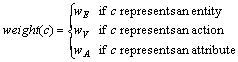
where wE, wV, and wA are positive constants that express the relative importance of the entities, actions, and attributes respectively. Their values are user-specified. In the future, a less arbitrary mechanism for assigning weights can be developed.
The function b (![]() ,
,![]() ) can be interpreted as a measure of the semantic similarity
between the concepts
) can be interpreted as a measure of the semantic similarity
between the concepts ![]() and
and ![]() . Currently we calculate it as follows:[4]
. Currently we calculate it as follows:[4]
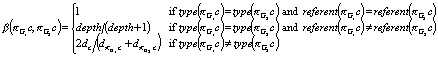
In the first condition, the concepts ![]() and
and ![]() are the same and thus
b (
are the same and thus
b (![]() ,
,![]() ) = 1.
) = 1.
In the second condition, the concepts ![]() and
and ![]() refer to different
individuals of the same type, i.e., different instances of the same class. In
this case,
refer to different
individuals of the same type, i.e., different instances of the same class. In
this case, ![]() , where depth
indicates the number of levels of the is-a
hierarchy. Using this value, the similarity between two concepts having the
same type but different referents is always greater that the similarity between
any two concepts with different types.
, where depth
indicates the number of levels of the is-a
hierarchy. Using this value, the similarity between two concepts having the
same type but different referents is always greater that the similarity between
any two concepts with different types.
In the third condition, the concepts ![]() and
and ![]() have different types,
i.e., refer to elements of different classes. In this case, we defineb(
have different types,
i.e., refer to elements of different classes. In this case, we defineb(![]() ,
,![]() ) as the semantic similarity between type(
) as the semantic similarity between type(![]() ) and type(
) and type(![]() ) in the is-a
hierarchy. We calculate it using a similar expression to one proposed in [11].
In this third option of our formula, di
indicates the distance – number of nodes – from the type i to the root of the hierarchy.
) in the is-a
hierarchy. We calculate it using a similar expression to one proposed in [11].
In this third option of our formula, di
indicates the distance – number of nodes – from the type i to the root of the hierarchy.
The relational similarity sr expresses how similar the relations among the common concepts in the conceptual graphs G1 and G2 are. In other words, the relational similarity indicates how similar the neighbors of the overlap in both original graphs are (see more details in [13]). We define the immediate neighbor of the overlap O in a conceptual graph Gi, NO(Gi), as the set of all the relations connected to the common concepts in the graph Gi:
![]() .
.
With this, we calculate the relational similarity sr using the following expression – also analogous to the Dice coefficient:
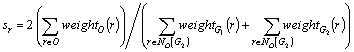
Here weightG(r) indicates the relative importance of the conceptual relation r in the conceptual graph G.[5] This value is calculated by the neighbor of the relation r. This kind of assignment guarantees the homogeneity between the concept and the relation weights. Hence, we compute weightG(r) as:
![]() .
.
Now that we have defined the two components
of the similarity measure, sc
and sr, we combine them
into a cumulative measure s. First,
the combination should be roughly multiplicative, for the cumulative measure to
be proportional to each of the two components. This would give the formula ![]() . However, we note that the relational similarity has a
secondary importance, because its existence depends on the existence of some
common concept nodes and because even if no common relations exist between the
common concepts of the two graphs, there exists some level of similarity
between them. Thus, while the cumulative similarity measure is proportional to sc, it still should not be
zero when sr = 0. So we
smooth the effect of sr
using the expression:
. However, we note that the relational similarity has a
secondary importance, because its existence depends on the existence of some
common concept nodes and because even if no common relations exist between the
common concepts of the two graphs, there exists some level of similarity
between them. Thus, while the cumulative similarity measure is proportional to sc, it still should not be
zero when sr = 0. So we
smooth the effect of sr
using the expression:
![]()
With this definition, if no relational similarity exists between the two graphs (sr = 0) then the general similarity only depends on the value of the conceptual similarity. In this situation, the general similarity is a fraction of the conceptual similarity, where the coefficient a indicates the value of this fraction.
The coefficients a and b reflect user-specified balance (0 < a, b < 1, a + b = 1). The coefficient a indicates the importance of the part of the similarity exclusively dependent on the common concepts and the coefficient b expresses the importance of the part of the similarity related with the connection of these common concepts. The user’s choice of a (and thus b) allows adjusting the similarity measure to the different applications and user interests. For instance, when a > b, the conceptual similarities are emphasized, while when b > a, stresses structural similarities.
4. An illustrative example
Our method for comparison of two conceptual graphs is very flexible. On one hand, it describes qualitatively and quantitatively the similarity between the two graphs. On the other hand, it considers the user interests all along the comparison process.
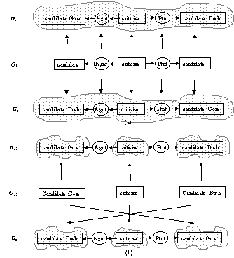
To illustrate this flexibility, we compare here two simple conceptual graphs. The first one represents the phrase “Gore criticizes Bush” and the second one the phrase “Bush criticizes Gore”.[6] The figure 4 shows the matching of these two graphs. Notice that their similarity can be described in two different ways, i.e., by two different and independent overlaps. The overlap O1 indicates that in both graphs “a candidate criticizes another candidate”, while the overlap O2 indicates that both graphs talk about Bush, Gore, and an action of criticizing.
The selection of the best overlap, i.e., the most appropriate description of the similarity, depends on the application and the user interests. These two parameters are modeled by the similarity measure. Table 1 shows the results for the comparison of these two conceptual graphs. Each result corresponds to a different way of evaluating and visualizing the similarity of these graphs. For instance, the first case emphasizes the structural similarity, the second one the conceptual similarity, and the third one focuses on the entities. In each case, the best overlap and the longer similarity measure are highlighted.
5. Conclusions
In order to start using more complete representations of texts than just keywords in the various applications of text processing, one of the main prerequisites is to have an appropriate method for the comparison of such new representations.
We considered representation of the texts by conceptual graphs and proposed a method for comparison of any pair of conceptual graphs. This method works in two main stages: matching conceptual graphs and measuring their similarity. Matching is mainly based on the generalization rules of conceptual graph theory. Similarity measure is based on the idea of the Dice coefficient but it also incorporates some new characteristics derived from the conceptual graph structure, for instance, the combination of two complementary sources of similarity: conceptual and relational similarity.
|
Figure 4. Flexible matching of two conceptual graphs |
Our method has two interesting characteristics. First, it uses domain knowledge, and second, it allows a direct influence of the user.
|
Table 1. The flexibility of the similarity measure
|
The domain knowledge is expressed in the form of a thesaurus and a set of small (shallow) is-a hierarchies, both customized by a specific user. The thesaurus allows considering the similarity between semantically related concepts, not necessarily equal, while the is-a hierarchies allow determining the similarities at different levels of generalization.
The flexibility of the method comes from the user-defined parameters. These allow analyzing the similarity of the two conceptual graphs from different points of view and also selecting the best interpretation in accordance with the user interests.
Because of this flexibility, our method can be used in different application areas of text processing, for instance, in information retrieval, textual case-based reasoning, and text mining. Currently, we are designing a method for the conceptual clustering of conceptual graphs based on these ideas and an information retrieval system where the non-topical information is represented by conceptual graphs.
References
1. Agrawal, Rakesh, and Ramakrishnan Srikant (1994), “Fast Algorithms for Mining Association Rules”, Proc. 20th VLDB Conference, Santiago de Chile, 1994.
2. Ellis and Lehmann (1994), “Exploiting the Induced Order on Type-Labeled Graphs for fast Knowledge Retrieval”, Lecture Notes in Artificial Intelligence 835, Springer-Verlag 1994.
3. Genest D., and M. Chein (1997). “An Experiment in Document Retrieval Using Conceptual Graphs”. Conceptual structures: Fulfilling Peirce´s Dream. Lecture Notes in artificial Intelligence 1257, August 1997.
4. Huibers, Ounis and Chevallet (1996), “Conceptual Graph Aboutness”, Lecture Notes in Artificial Intelligence, Springer, 1996.
5. Marie, Marie (1995), “On generalization / specialization for conceptual graphs”, Journal of Experimental and Theoretical Artificial Intelligence, volume 7, pages 325-344, 1995.
6. Myaeng, Sung H., and Aurelio López-López (1992), “Conceptual Graph Matching: a Flexible Algorithm and Experiments”, Journal of Experimental and Theoretical Artificial Intelligence, Vol. 4, 1992.
7. Myaeng, Sung H. (1992). “Using Conceptual graphs for Information Retrieval: A Framework for Adequate Representation and Flexible Inferencing”, Proc. of Symposium on Document Analysis and Information Retrieval, Las Vegas, 1992.
8. Rasmussen, Edie (1992). “Clustering Algorithms”. Information Retrieval: Data Structures & Algorithms. William B. Frakes and Ricardo Baeza-Yates (Eds.), Prentice Hall, 1992.
9. Sowa, John F. (1984). “Conceptual Structures: Information Processing in Mind and Machine”. Ed. Addison-Wesley, 1984.
10. Sowa, John F. (1999). “Knowledge Representation: Logical, Philosophical and Computational Foundations”. 1st edition, Thomson Learning, 1999.
11. Wu and Palmer (1994), “Verb Semantics and Lexical Selection”, Proc. of the 32nd Annual Meeting of the Associations for Computational Linguistics, 1994.
12. Yang, Choi and Oh (1992), “CGMA: A Novel Conceptual Graph Matching Algorithm”, Proc. of the 7th Conceptual Graphs Workshop, Las Cruces, NM, 1992.
13. Manuel Montes-y-Gómez, Alexander Gelbukh, Aurelio López-López (2000). Comparison of Conceptual Graphs. O. Cairo, L.E. Sucar, F.J. Cantu (eds.) MICAI 2000: Advances in Artificial Intelligence. Lecture Notes in Artificial Intelligence N 1793, Springer-Verlag, pp. 548-556, 2000.
14. A. F. Gelbukh. “Review of R. Hausser’s ‘Foundations of Computational Linguistics: Man-Machine Communication in Natural Language’.” Computational Linguistics, 26 (3), 2000.
15. Manuel Montes-y-Gómez, Aurelio López-López, and Alexander Gelbukh. Information Retrieval with Conceptual Graph Matching. Proc. DEXA-2000, 11th International Conference on Database and Expert Systems Applications, Greenwich, England, September 4-8, 2000. Lecture Notes in Computer Science N 1873, Springer-Verlag, pp. 312–321.